Decision Trees¶

After linear regression, decision trees are probably the second most commonly known model used for regression. Decision trees are completely different from linear regression, in that they are not represented by an equation. They are still functions (mathematically-speaking), because a function is just a rule which assigns an output given an input. But the function looks completely different from what you’re used to.

Below is an example of a decision tree being used to determine whether or not a passenger on the Titanic would survive:

Titanic Decision Tree

We refer to each “question” in the tree (e.g. “Is age > 9.5?”) as a “leaf” or “node”. A question you may be wondering is, how do we know what questions we should be asking at each leaf? Also, what should the cutoff be for each question? Why are we asking about age being greater than 9.5 instead of 10, 11, or something else altogether? The answer is, decision trees automatically learn what questions to ask in order to generate the best possible predictions. Let’s jump in and start exploring.

Imports¶

import pandas as pd
import numpy as np

from matplotlib import pyplot as plt

from sklearn.model_selection import train_test_split
from sklearn.preprocessing import LabelEncoder

Loading data¶

For this project we’ll be working with the finishing times for male runners in the LA Marathon. We’ll be training on model on 2016, and testing it on 2017. I scraped the data from the official results site.

df = pd.read_csv('data/2016_la_marathon.csv')

df.head()

	div_place	name	bib	age	place	gender_place	5k_split	10k_split	15k_split	20k_split	25k_split	30k_split	35k_split	40k_split	clock_time	net_time	hometown
0	1	SAUL VISCARRA	40402	15	382	352	22:28	44:00	1:04:56	1:26:24	1:48:24	2:11:32	2:37:42	3:01:56	3:22:41	3:11:51	NaN
1	2	FERNANDO GOMEZ	40504	15	560	504	22:37	45:17	1:07:50	1:31:42	1:55:46	2:19:58	2:44:35	3:09:32	3:23:09	3:18:54	NaN
2	3	MARCOS GONZALEZ	40882	15	1042	881	24:08	47:44	1:10:34	1:34:10	1:58:40	2:23:37	2:54:01	3:23:20	3:43:35	3:31:59	NaN
3	4	LUIS MORALES	42286	13	1294	1076	22:50	46:21	1:11:07	1:34:42	1:58:49	2:24:17	2:54:27	3:26:22	3:41:55	3:37:24	NaN
4	5	PETER CASTANO	20099	15	1413	1166	26:13	53:12	1:19:36	1:45:47	2:11:53	2:38:18	3:03:38	3:29:46	3:45:48	3:39:31	NaN

Data preparation¶

Let’s start with our usual check of NaN/None values.

for col in df.columns:
    missing_value_count = df[col].isna().sum()
    print(f'{col}: {missing_value_count} missing')

div_place: 0 missing
name: 0 missing
bib: 0 missing
age: 0 missing
place: 0 missing
gender_place: 0 missing
5k_split: 821 missing
10k_split: 158 missing
15k_split: 101 missing
20k_split: 91 missing
25k_split: 73 missing
30k_split: 140 missing
35k_split: 95 missing
40k_split: 161 missing
clock_time: 0 missing
net_time: 0 missing
hometown: 11499 missing

It looks like a number of them are missing. This could be from people dropping out of the race, never showing up, etc. Since we’re trying to predict finishing time, let’s drop any rows which having a missing split.

split_columns = ['5k_split', '10k_split', '15k_split', '20k_split', '25k_split', '30k_split', '35k_split', '40k_split']

df = df.dropna(how='any', subset=split_columns)

We want to predict the runners placing based on their how fast they run, along with potentially some other information. Currently, their splits (times) at each 5 kilometers is written in the form hours:minutes:seconds. That’s not really what we want, we need numbers to work with. So we’ll start by converting those values to minutes. To do so we’ll use the Pandas .apply() function, which takes in a function, and applies it to each row individually.

Let’s write our function to look for the ‘:’ character, and then split at it. Note that depending on how fast/slow the runner was, there could be more than one colon in their time (for hours:minutes:seconds versus just minutes:seconds). So we’ll need to check the length of our list and process each part individually. To convert seconds into minutes we’ll divide by 60, and to convert hours into minutes we’ll multiply by 60. Finally, since we’re starting with a string, when we split it, we will again receive strings. Let’s do a simple test case first to make sure we have the idea.

speed_split = '23:45'.split(':')
print(f'The value {speed_split[0]} is a {type(speed_split[0])}')
print(f'The value {speed_split[1]} is a {type(speed_split[1])}')

The value 23 is a <class 'str'>
The value 45 is a <class 'str'>

This works, but if we’re going to do math, we need integers, not strings. So we’ll convert each to an integer as well.

speed_split = '23:45'.split(':')
print(f'The value {int(speed_split[0])} is a {type(int(speed_split[0]))}')
print(f'The value {int(speed_split[1])} is a {type(int(speed_split[1]))}')

The value 23 is a <class 'int'>
The value 45 is a <class 'int'>

Let’s now write our function to take in an arbitrary speed (written as a string), split it up, convert it to minutes, and return it.

def split_to_minutes(speed):
    speed_split = speed.split(':')
    # If there's only one colon, so minutes:seconds
    if len(speed_split) == 2:
        minutes = int(speed_split[0]) + int(speed_split[1])/60
    # If there's two colon, so hours:minutes:seconds
    if len(speed_split) == 3:
        minutes = 60*int(speed_split[0]) + int(speed_split[1]) + int(speed_split[2])/60
    return minutes

Let’s test it.

split_to_minutes('10:35')

10.583333333333334

With that, we can now apply our function to our dataframe. It’s good practice to not overwrite a column in a dataframe, because maybe you’ll need it later. So we’ll create a new column for each 5 kilometers, titled 5k_split_min, 10k_split_min, etc., as well as any other columns with times in them. We could go through and do this one at a time, but by using a for loop we can save ourselves time.

# An error is coming...
time_columns = ['5k_split', '10k_split', '15k_split', '20k_split', '25k_split', '30k_split', '35k_split', '40k_split', 'clock_time', 'net_time']

for col in time_columns:
    df[f'{col}_min'] = df[col].apply(split_to_minutes)

---------------------------------------------------------------------------
ValueError                                Traceback (most recent call last)
<ipython-input-11-23ed3fc323d1> in <module>
      3 
      4 for col in time_columns:
----> 5     df[f'{col}_min'] = df[col].apply(split_to_minutes)

~/anaconda3/envs/math_3439/lib/python3.8/site-packages/pandas/core/series.py in apply(self, func, convert_dtype, args, **kwds)
   3846             else:
   3847                 values = self.astype(object).values
-> 3848                 mapped = lib.map_infer(values, f, convert=convert_dtype)
   3849 
   3850         if len(mapped) and isinstance(mapped[0], Series):

pandas/_libs/lib.pyx in pandas._libs.lib.map_infer()

<ipython-input-9-0f784b837919> in split_to_minutes(speed)
      3     # If there's only one colon, so minutes:seconds
      4     if len(speed_split) == 2:
----> 5         minutes = int(speed_split[0]) + int(speed_split[1])/60
      6     # If there's two colon, so hours:minutes:seconds
      7     if len(speed_split) == 3:

ValueError: invalid literal for int() with base 10: '0-33'

Oh no! Reading the error, it looks like someone has a time of ‘0-33’ which is causing issues when we try to convert it to an integer. So perhaps we should modify our function to first check for a valid value, and if it’s not valid, to just fill in a None. Then we can drop rows with None afterward. To do so, we’ll use the Python pattern try…except…. What this does is to try and do what you ask, but if an error occurs, rather than just crashing and throwing the error, it enters the except block. You can then make something else happen in there, like filling in a None.

def split_to_minutes(speed):
    speed_split = speed.split(':')
    for value in speed_split:
        try:
            # Check if it can be converted to an integer. If it can't, this will fail and Python will proceed to the "except" part
            int(value)
        except Exception as e:
            return None
    # This part below is just the function we wrote above
    if len(speed_split) == 2:
        minutes = int(speed_split[0]) + int(speed_split[1])/60
    if len(speed_split) == 3:
        minutes = 60*int(speed_split[0]) + int(speed_split[1]) + int(speed_split[2])/60
    return minutes

split_columns = ['5k_split', '10k_split', '15k_split', '20k_split', '25k_split', '30k_split', '35k_split', '40k_split']
time_columns = split_columns + ['clock_time', 'net_time']

for col in time_columns:
    df[f'{col}_min'] = df[col].apply(split_to_minutes)

df.head()

	div_place	name	bib	age	place	gender_place	5k_split	10k_split	15k_split	20k_split	...	5k_split_min	10k_split_min	15k_split_min	20k_split_min	25k_split_min	30k_split_min	35k_split_min	40k_split_min	clock_time_min	net_time_min
0	1	SAUL VISCARRA	40402	15	382	352	22:28	44:00	1:04:56	1:26:24	...	22.466667	44.000000	64.933333	86.400000	108.400000	131.533333	157.700000	181.933333	202.683333	191.850000
1	2	FERNANDO GOMEZ	40504	15	560	504	22:37	45:17	1:07:50	1:31:42	...	22.616667	45.283333	67.833333	91.700000	115.766667	139.966667	164.583333	189.533333	203.150000	198.900000
2	3	MARCOS GONZALEZ	40882	15	1042	881	24:08	47:44	1:10:34	1:34:10	...	24.133333	47.733333	70.566667	94.166667	118.666667	143.616667	174.016667	203.333333	223.583333	211.983333
3	4	LUIS MORALES	42286	13	1294	1076	22:50	46:21	1:11:07	1:34:42	...	22.833333	46.350000	71.116667	94.700000	118.816667	144.283333	174.450000	206.366667	221.916667	217.400000
4	5	PETER CASTANO	20099	15	1413	1166	26:13	53:12	1:19:36	1:45:47	...	26.216667	53.200000	79.600000	105.783333	131.883333	158.300000	183.633333	209.766667	225.800000	219.516667

5 rows × 27 columns

Looking good! Let’s see where None’s occurred as a result of bad values.

for col in df.columns:
    missing_value_count = df[col].isna().sum()
    print(f'{col} - {missing_value_count} missing')

div_place - 0 missing
name - 0 missing
bib - 0 missing
age - 0 missing
place - 0 missing
gender_place - 0 missing
5k_split - 0 missing
10k_split - 0 missing
15k_split - 0 missing
20k_split - 0 missing
25k_split - 0 missing
30k_split - 0 missing
35k_split - 0 missing
40k_split - 0 missing
clock_time - 0 missing
net_time - 0 missing
hometown - 10375 missing
5k_split_min - 4 missing
10k_split_min - 0 missing
15k_split_min - 0 missing
20k_split_min - 0 missing
25k_split_min - 0 missing
30k_split_min - 0 missing
35k_split_min - 0 missing
40k_split_min - 0 missing
clock_time_min - 0 missing
net_time_min - 0 missing

Looks like just a couple in 5k_split_min. Let’s drop and we should be good to go!

df = df.dropna(how='any', subset=['5k_split_min'])

df.shape

(10371, 27)

So we still have over 10,000 runners left to work with, that should be plenty for our purposes. With our data prepped, let’s start modeling.

Decision trees ¶

Let’s just jump right in and use sklearn’s implementation of DecisionTree. We want to predict their placing, so this is a regression problem, because we are predicting a continuous value. While placing is not really continuous (no one could get 4.3 place), there are so many possible values that it would be ridiculous to have a different category for each place. Therefore, it makes more sense to think of it as being continuous than as being categorical. Decision trees can be used for both regression and classification. They are more commonly used for classification, but we’ll start by using it for regression. To do so we will be using DecisionTreeRegressor from sklearn. Training it and making predictions with it should look exactly like how we did for linear regression. Let’s use all of our splits to predict their finishing place. We said we’ll test on 2017, but let’s still split 2016 into two sets in order to have something to tune our model with. Since 2017 is our true “test” data, it doesn’t make sense to say we’re splitting 2016 into train and “test” data. Thus subsetting the data this way is referred to as creating a “validation set”. A validation set is used to tweak your model until you’re ready to actually test it. It’s best practice to keep your test data as true test data, and not “show it” to your model before your model is ready.

from sklearn.model_selection import train_test_split

# Our new split columns are named the same as the old split column, but with "_min" appended. So let's create a list of those.
split_columns_min = [f'{x}_min' for x in split_columns]
split_cols_and_age = split_columns_min + ['age']

X_train, X_valid, y_train, y_valid = train_test_split(df[split_cols_and_age], df['gender_place'], train_size=0.7)

X_train.head()

	5k_split_min	10k_split_min	15k_split_min	20k_split_min	25k_split_min	30k_split_min	35k_split_min	40k_split_min	age
2111	36.450000	68.966667	98.183333	129.983333	163.216667	203.983333	246.666667	286.816667	22
8256	27.916667	55.066667	82.016667	108.916667	139.033333	166.833333	201.250000	232.483333	46
4209	29.833333	60.433333	90.866667	123.050000	154.800000	187.750000	222.083333	255.266667	30
5336	22.366667	44.883333	67.383333	89.833333	112.233333	135.733333	166.750000	200.400000	38
11394	29.583333	60.600000	90.250000	120.016667	150.650000	181.816667	213.216667	244.083333	72

Using a decision tree in sklearn is exactly like how you’ve used all other models in sklearn! From the perspective of someone learning machine learning, one of the best features about sklearn is how consistent it is. Pretty much every model follows the same pattern:

Instantiate the model (meaning something like lr = LinearRegression() or clf = LogisticRegression().
Fit the model using .fit()
Use the model to make predictions using .predict()
(Optional) Get the score of the model (usually R^2 for regression and accuracy for classification) using .score()

Let’s follow this same pattern here.

from sklearn.tree import DecisionTreeRegressor

dt_reg = DecisionTreeRegressor()

dt_reg.fit(X_train, y_train)

DecisionTreeRegressor(ccp_alpha=0.0, criterion='mse', max_depth=None,
                      max_features=None, max_leaf_nodes=None,
                      min_impurity_decrease=0.0, min_impurity_split=None,
                      min_samples_leaf=1, min_samples_split=2,
                      min_weight_fraction_leaf=0.0, presort='deprecated',
                      random_state=None, splitter='best')

preds = dt_reg.predict(X_valid)

for i in range(10):
    print(f'Predicted: {preds[i]}, Actual: {y_valid.iloc[i]}, Diff = {preds[i]-y_valid.iloc[i]} ({100*abs(preds[i]-y_valid.iloc[i])/y_valid.iloc[i]:.2f}%)')

Predicted: 2506.0, Actual: 2545, Diff = -39.0 (1.53%)
Predicted: 800.0, Actual: 847, Diff = -47.0 (5.55%)
Predicted: 10298.0, Actual: 10197, Diff = 101.0 (0.99%)
Predicted: 8833.0, Actual: 8577, Diff = 256.0 (2.98%)
Predicted: 10989.0, Actual: 10828, Diff = 161.0 (1.49%)
Predicted: 1959.0, Actual: 1890, Diff = 69.0 (3.65%)
Predicted: 10721.0, Actual: 10694, Diff = 27.0 (0.25%)
Predicted: 1368.0, Actual: 1328, Diff = 40.0 (3.01%)
Predicted: 2193.0, Actual: 2157, Diff = 36.0 (1.67%)
Predicted: 1674.0, Actual: 1724, Diff = -50.0 (2.90%)

So most of these predictions are within a handful of percent (50-ish places) of being correct, that’s impressive! For comparison, let’s also build a linear regressor with this same data and compare the MSE from both.

from sklearn.linear_model import LinearRegression

lr = LinearRegression()

lr.fit(X_train, y_train)

LinearRegression(copy_X=True, fit_intercept=True, n_jobs=None, normalize=False)

preds_lr = lr.predict(X_valid)

for i in range(10):
    print(f'Predicted: {preds_lr[i]}, Actual: {y_valid.iloc[i]}, Diff = {preds_lr[i]-y_valid.iloc[i]} ({100*abs(preds_lr[i]-y_valid.iloc[i])/y_valid.iloc[i]:.2f}%)')

Predicted: 2881.4505952084746, Actual: 2545, Diff = 336.4505952084746 (13.22%)
Predicted: 1019.8154901168928, Actual: 847, Diff = 172.81549011689276 (20.40%)
Predicted: 9987.114569245616, Actual: 10197, Diff = -209.8854307543843 (2.06%)
Predicted: 8196.702056815542, Actual: 8577, Diff = -380.29794318445784 (4.43%)
Predicted: 11653.02324126436, Actual: 10828, Diff = 825.02324126436 (7.62%)
Predicted: 2274.0219966673267, Actual: 1890, Diff = 384.0219966673267 (20.32%)
Predicted: 11318.176668353688, Actual: 10694, Diff = 624.176668353688 (5.84%)
Predicted: 1798.1529686199756, Actual: 1328, Diff = 470.1529686199756 (35.40%)
Predicted: 2442.903099096622, Actual: 2157, Diff = 285.9030990966221 (13.25%)
Predicted: 2144.7100749666715, Actual: 1724, Diff = 420.7100749666715 (24.40%)

The tree model looks to have done much better! Let’s compare R^2 and MSE to be sure.

print(f'Decision tree R^2 = {dt_reg.score(X_valid, y_valid)**2}')
print(f'Linear regression R^2 = {lr.score(X_valid, y_valid)**2}')

Decision tree R^2 = 0.9972689036020543
Linear regression R^2 = 0.9579743493585986

from sklearn.metrics import mean_squared_error as mse

print(f'Linear regresion MSE = {mse(preds_lr, y_valid)}')
print(f'Decision Tree MSE = {mse(preds, y_valid)}')

Linear regresion MSE = 231799.09438088024
Decision Tree MSE = 14914.017030848328

That’s a huge difference!

We said that a decision tree makes decisions by learning to split each leaf at a particular value. So what decisions did our tree learn to make? To answer that we can visualize our tree. sklearn has a built-in function called plot_tree. Warning: Plotting this will take a while…

from sklearn.tree import plot_tree

plt.figure(figsize=(12, 8))
plot_tree(dt);

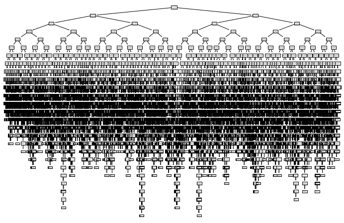
Overfitting and hyperparameters ¶

Woah, what happened there!? It looks like our tree is incredibly complex, with many, many different pathways and conditions. That’s not really what we want, because it’s likely the case that our model is overfitting. By overfitting we mean developing an overly complex model which does not generalize well to other scenarios. So it’s likely that the super-specific rules it learned will not apply well to 2017, nor any other year.

When building a tree there are various hyperparameters that are used to control how the tree is grown. By hyperparameters we mean the values in a model that must be chosen by the user (as opposed to being learned from the data). The most common hyperparameters for decision trees are the following:

max_depth: Controls how many levels the tree can have (so max_depth=1 means only one “question” can be asked to split the tree).
min_samples_split: Controls how many samples need to be seen which satisfy a rule before a new rule can be created. So if only two runners have a 5k split faster than 20 minutes (say), then by setting min_samples_split=3 (or anything bigger than 2), no new rules would be created for these runners. This helps avoid creating ultra-specific nodes which may not generalize well.
max_features: How many columns can be considered. Again, this controls creating super-specific rules that require many, many columns to satisfy.

Let’s look at the depth and number of leaves of the tree we just built.

print(f'Depth = {dt.get_depth()}')
print(f'# of leaves = {dt.get_n_leaves()}')

Depth = 26
# of leaves = 7259

So our decision tree had thousands of different “rules” (i.e. leaves). Since we only had a little over 10k runners, this means most runners had their own individual rule! This is a problem, because we want to build a model that would work in general, not just on the data we trained it on. However, our tree instead learned a specific rule for every 1 or 2 runners. This could be something like “if their 5k time was less than 48 minutes and their 10k time was greater than 60 minutes and their 15k was less than… then predict 5920’th place”. This is what we mean by “overfitting”.

The way to avoid overfitting is to restrict our tree by picking hyperparameters that do not allow ultra-specific rules to be learned. Let’s try building our tree again, but starting with some very mild hyperparameter choices to avoid this phenomenon of having an overly-complex tree. To do so, you simply need to supply these hyperparameters to the decision tree when you instantiate it (step 1).

dt_simple = DecisionTreeRegressor(max_depth=3, min_samples_split=5)

dt_simple.fit(X_train, y_train)

preds_simple = dt_simple.predict(X_valid)

Let’s plot this decision tree as well to see what it’s like.

plt.figure(figsize=(20,10))
plot_tree(dt_simple, feature_names=split_columns_min);

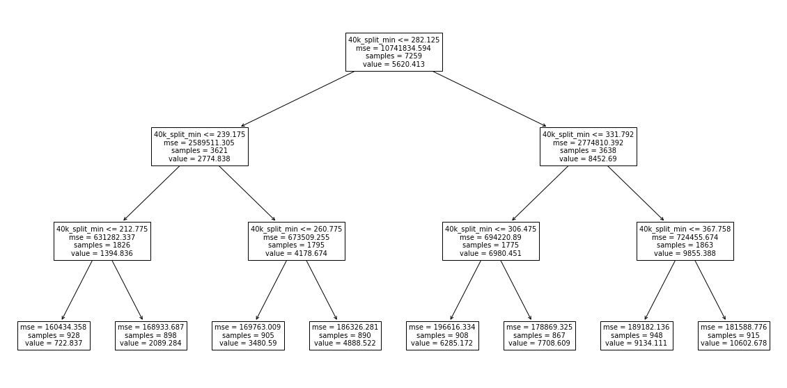
So we can see that it begins by looking at the 40k_split_min time, splits it at 282.125 minutes, and then makes other decisions based on that. This seems like a more reasonable way to design a tree.

We’d like to evaluate how well our model did. We’ve been doing that by putting some print statements inside a for loop, and also computing the MSE. Rather than continuing to copy-and-paste that code, let’s create a function which does it for us.

def summarize_model(preds, actual, num_examples=10):
    if isinstance(actual, pd.Series):
        actual = actual.values
        
    for i in range(num_examples):
        print(f'Predicted: {preds[i]:.2f}, Actual: {actual[i]:.2f}, Diff = {preds[i]-actual[i]:.2f} ({100*abs(preds[i]-actual[i])/actual[i]:.2f}%)')
        
    print()
    print(f'MSE: {mse(preds, actual)}')

summarize_model(preds_simple, y_valid)

Predicted: 2089.28, Actual: 2545.00, Diff = -455.72 (17.91%)
Predicted: 722.84, Actual: 847.00, Diff = -124.16 (14.66%)
Predicted: 10602.68, Actual: 10197.00, Diff = 405.68 (3.98%)
Predicted: 9134.11, Actual: 8577.00, Diff = 557.11 (6.50%)
Predicted: 10602.68, Actual: 10828.00, Diff = -225.32 (2.08%)
Predicted: 2089.28, Actual: 1890.00, Diff = 199.28 (10.54%)
Predicted: 10602.68, Actual: 10694.00, Diff = -91.32 (0.85%)
Predicted: 722.84, Actual: 1328.00, Diff = -605.16 (45.57%)
Predicted: 2089.28, Actual: 2157.00, Diff = -67.72 (3.14%)
Predicted: 2089.28, Actual: 1724.00, Diff = 365.28 (21.19%)

MSE: 181762.05746029768

Not great, but we also drastically reduced the complexity of our decision tree, so that’s to be expected. Also, notice that with only a very mild tree structure, our MSE of 182,162 is still lower than the MSE from linear regression of 220,525.

Let’s also plot the predictions made by the tree against the actual, correct values. On both the x- and y-axis we’ll put the place the person got. This might seem weird, as normally the x-axis is what we feed into our model. But since we’re feeding so many variables into our model, there’s no single one to put on the x-axis. By putting the placing on both the x- and y-axis, a perfect prediction will be a diagonal line. However, our model is not perfect, so any deviation from that will let us see what’s going on.

plt.figure(figsize=(12,8))
plt.scatter(x=y_valid, y=y_valid, color='blue', label='Actual')
plt.scatter(x=y_valid, y=preds_simple, color='red', label='Predicted')
plt.legend();

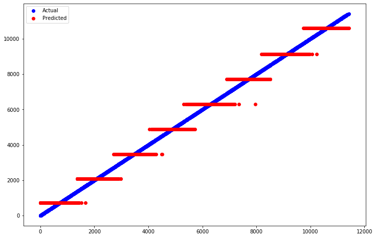
So it looks like our tree is roughly learning a step-function. In fact, if you look above at the tree diagram, you’ll see that each leaf on the bottom row tells you exactly what value it will predict for the placing for every runner who satisfied the necessary conditions to end up in that leaf. For example, to get to the first leaf on the left (starting at the top of the tree), a runner must have:

Had a 40k split of less than 282 minutes
Had a 40k split of less than 239 minutes
Had a 40k split less than 212 minutes they would be assigned a finishing place of 722. Apparently there were 928 such runners (samples). WARNING: Your numbers may vary, as decision trees involve randomness, and each run will produce new results unless random_state is specified when building the tree.

So wait a minute, every leaf in the tree is just looking at the 40k split! Why is that? Probably because that’s the last split just 2 kilometers before the finishing line. So obviously the top finishers would be the fastest to that point! This is an example of building a model without really thinking about your data. If you’re not careful you can easily get results which seem good, but upon closer inspection they are highly flawed.

To build a more realistic and useful model, let’s restrict ourselves to just the earlier splits to have a less-obvious problem. Let’s take the first three splits (5k, 10k and 15k), along with their age. Again, let’s first apply linear regression as a baseline. If our more complicated tree model can’t beat a simple line, then we’re doing something wrong.

# Grab just these columns in the training and validation sets
# Note that the y doesn't change, because y is just their place, nothing to do with their times
splits_5_10_15_age_cols = ['5k_split_min', '10k_split_min', '15k_split_min', 'age']

X_train_splits_5_10_15_age = X_train[splits_5_10_15_age_cols]
X_valid_splits_5_10_15_age = X_valid[splits_5_10_15_age_cols]

# Fit a linear regression model
lr_splits_5_10_15_age = LinearRegression()
lr_splits_5_10_15_age.fit(X_train_splits_5_10_15_age, y_train)

LinearRegression(copy_X=True, fit_intercept=True, n_jobs=None, normalize=False)

# Fit a decision tree
dt_splits_5_10_15_age = DecisionTreeRegressor(max_depth=3, min_samples_split=5)
dt_splits_5_10_15_age.fit(X_train_splits_5_10_15_age, y_train)

DecisionTreeRegressor(ccp_alpha=0.0, criterion='mse', max_depth=3,
                      max_features=None, max_leaf_nodes=None,
                      min_impurity_decrease=0.0, min_impurity_split=None,
                      min_samples_leaf=1, min_samples_split=5,
                      min_weight_fraction_leaf=0.0, presort='deprecated',
                      random_state=None, splitter='best')

# Make predictions on the validation set with both the decision tree and the linear regression model
lr_splits_5_10_15_age_preds = lr_splits_5_10_15_age.predict(X_valid_splits_5_10_15_age)
dt_splits_5_10_15_age_preds = dt_splits_5_10_15_age.predict(X_valid_splits_5_10_15_age)

# Results for linear regression
print('Linear model:')
print('='*20)
summarize_model(lr_splits_5_10_15_age_preds, y_valid)

Linear model:
====================
Predicted: 2594.78, Actual: 2545.00, Diff = 49.78 (1.96%)
Predicted: 1791.78, Actual: 847.00, Diff = 944.78 (111.54%)
Predicted: 10640.01, Actual: 10197.00, Diff = 443.01 (4.34%)
Predicted: 8094.84, Actual: 8577.00, Diff = -482.16 (5.62%)
Predicted: 6810.22, Actual: 10828.00, Diff = -4017.78 (37.11%)
Predicted: 3196.10, Actual: 1890.00, Diff = 1306.10 (69.11%)
Predicted: 10615.06, Actual: 10694.00, Diff = -78.94 (0.74%)
Predicted: 2054.87, Actual: 1328.00, Diff = 726.87 (54.73%)
Predicted: 2295.13, Actual: 2157.00, Diff = 138.13 (6.40%)
Predicted: 2694.68, Actual: 1724.00, Diff = 970.68 (56.30%)

MSE: 1674606.3773056634

# Results for the decision tree model
print('Decision tree model:')
print('='*20)
summarize_model(dt_splits_5_10_15_age_preds, y_valid)

Decision tree model:
====================
Predicted: 2168.25, Actual: 2545.00, Diff = -376.75 (14.80%)
Predicted: 779.43, Actual: 847.00, Diff = -67.57 (7.98%)
Predicted: 8884.37, Actual: 10197.00, Diff = -1312.63 (12.87%)
Predicted: 7413.37, Actual: 8577.00, Diff = -1163.63 (13.57%)
Predicted: 7413.37, Actual: 10828.00, Diff = -3414.63 (31.54%)
Predicted: 2168.25, Actual: 1890.00, Diff = 278.25 (14.72%)
Predicted: 10278.75, Actual: 10694.00, Diff = -415.25 (3.88%)
Predicted: 2168.25, Actual: 1328.00, Diff = 840.25 (63.27%)
Predicted: 2168.25, Actual: 2157.00, Diff = 11.25 (0.52%)
Predicted: 2168.25, Actual: 1724.00, Diff = 444.25 (25.77%)

MSE: 1648919.7445526074

So the decision tree actually did slightly worse this time. Let’s plot the predictions of both models against the actual values to get a feel for what’s going on.

plt.figure(figsize=(16,8))
plt.scatter(x=y_valid, y=y_valid, color='blue', label='Actual', alpha=0.2)
plt.scatter(x=y_valid, y=dt_splits_5_10_15_age_preds, color='green', label='DT Predicted', alpha=0.2)
plt.scatter(x=y_valid, y=lr_splits_5_10_15_age_preds, color='red', label='LR Predicted', alpha=0.2)

plt.xlabel('Actual placing')
plt.ylabel('Predicted placing')

lr_r2 = lr_splits_5_10_15_age.score(X_valid_splits_5_10_15_age, y_valid)**2
dt_r2 = dt_splits_5_10_15_age.score(X_valid_splits_5_10_15_age, y_valid)**2

plt.title(f'LR R^2 = {lr_r2:.3f}, DT R^2 = {dt_r2:.3f}')

plt.legend();

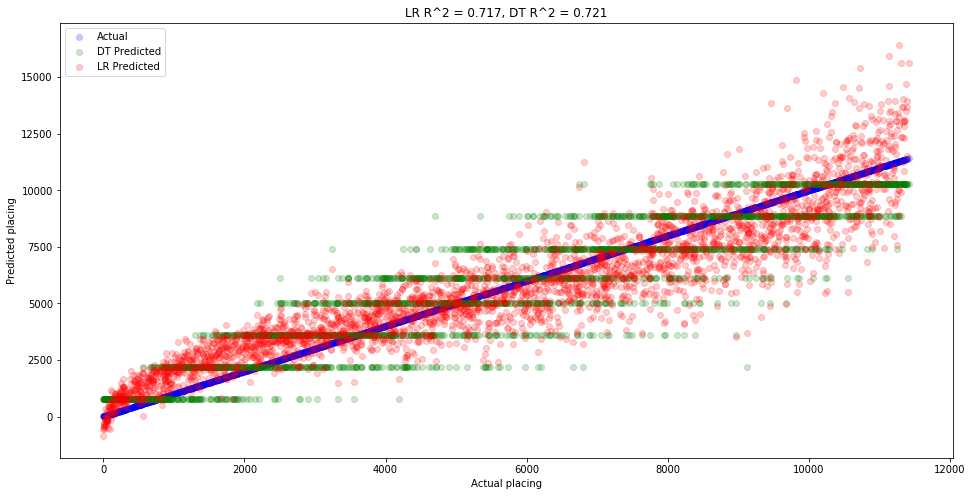
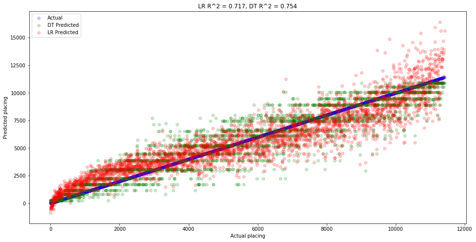
So again we see that the decision tree (green) is approximating a step function. You can see these values by going to the diagram we printed of our decision tree and looking at the leaves on the bottom row. Each one will say value=..., which is the value that gets assigned to that entire leaf. This is why decision trees are more often used for classification then regression. That’s because regression typically involves continuous values, whereas decision trees produce decidedly non-continuous step functions. Having said that, decision trees are extremely powerful and should not be overlooked for any type of problem.

Let’s build one last decision tree, this time with a medium-level of depth and complexity. The point is to see how complex our tree needs to be before it outpeforms linear regression.

# Create our tree
dt_splits_5_10_15_age2 = DecisionTreeRegressor(max_depth=5, min_samples_split=5)

# Train our tree
dt_splits_5_10_15_age2.fit(X_train_splits_5_10_15_age, y_train)

# Make predictions with our tree
dt_splits_5_10_15_age_preds2 = dt_splits_5_10_15_age2.predict(X_valid_splits_5_10_15_age)

# Compare predictions to linear regression
print('Linear model:')
print('='*20)
summarize_model(lr_splits_5_10_15_age_preds, y_valid)

print('Decision tree model:')
print('='*20)
summarize_model(dt_splits_5_10_15_age_preds2, y_valid)

# R^2
lr_r2 = lr_splits_5_10_15_age.score(X_valid_splits_5_10_15_age, y_valid)**2 # Same as above
dt_r2 = dt_splits_5_10_15_age2.score(X_valid_splits_5_10_15_age, y_valid)**2

# Plot the predictions
plt.figure(figsize=(16,8))
plt.scatter(x=y_valid, y=y_valid, color='blue', label='Actual', alpha=0.2)
plt.scatter(x=y_valid, y=dt_splits_5_10_15_age_preds2, color='green', label='DT Predicted', alpha=0.2)
plt.scatter(x=y_valid, y=lr_splits_5_10_15_age_preds, color='red', label='LR Predicted', alpha=0.2)

plt.xlabel('Actual placing')
plt.ylabel('Predicted placing')

plt.title(f'LR R^2 = {lr_r2:.3f}, DT R^2 = {dt_r2:.3f}')

plt.legend();

Linear model:
====================
Predicted: 2594.78, Actual: 2545.00, Diff = 49.78 (1.96%)
Predicted: 1791.78, Actual: 847.00, Diff = 944.78 (111.54%)
Predicted: 10640.01, Actual: 10197.00, Diff = 443.01 (4.34%)
Predicted: 8094.84, Actual: 8577.00, Diff = -482.16 (5.62%)
Predicted: 6810.22, Actual: 10828.00, Diff = -4017.78 (37.11%)
Predicted: 3196.10, Actual: 1890.00, Diff = 1306.10 (69.11%)
Predicted: 10615.06, Actual: 10694.00, Diff = -78.94 (0.74%)
Predicted: 2054.87, Actual: 1328.00, Diff = 726.87 (54.73%)
Predicted: 2295.13, Actual: 2157.00, Diff = 138.13 (6.40%)
Predicted: 2694.68, Actual: 1724.00, Diff = 970.68 (56.30%)

MSE: 1674606.3773056634
Decision tree model:
====================
Predicted: 1723.91, Actual: 2545.00, Diff = -821.09 (32.26%)
Predicted: 1182.63, Actual: 847.00, Diff = 335.63 (39.63%)
Predicted: 9469.34, Actual: 10197.00, Diff = -727.66 (7.14%)
Predicted: 7719.15, Actual: 8577.00, Diff = -857.85 (10.00%)
Predicted: 7719.15, Actual: 10828.00, Diff = -3108.85 (28.71%)
Predicted: 2252.04, Actual: 1890.00, Diff = 362.04 (19.16%)
Predicted: 10065.15, Actual: 10694.00, Diff = -628.85 (5.88%)
Predicted: 1723.91, Actual: 1328.00, Diff = 395.91 (29.81%)
Predicted: 1723.91, Actual: 2157.00, Diff = -433.09 (20.08%)
Predicted: 1723.91, Actual: 1724.00, Diff = -0.09 (0.01%)

MSE: 1440131.3709699702

We’ve learned a valuable lesson in this notebook, which is that just because a model gives better results, doesn’t mean it’s a better model. We saw this with the decision tree, where it gave great predictions, but the tree itself was so complicated that it seemed unrealistic. Does it really make sense to have a model which requires most individuals to have their own custom rule. This leads to overfitting, which means models that don’t generalize well. In the future, we’ll look at our data more closely before just blindly picking a model to apply.

The mathematics of decision trees ¶

While we’ve now discussed what a decision tree is, there is still the question of how a decision tree is made. How is it that sklearn decides which column to look at first, and what the cutoff should be? Let’s go back to the Titanic data to understand this.

df = pd.read_csv(drive_dir + 'data/titanic.csv')

df.head()

	PassengerId	Survived	Pclass	Name	Sex	Age	SibSp	Ticket	Fare	Cabin	Embarked
0	1	0	3	Braund, Mr. Owen Harris	male	22.0	1	A/5 21171	7.2500	NaN	S
1	2	1	1	Cumings, Mrs. John Bradley (Florence Briggs Th...	female	38.0	1	PC 17599	71.2833	C85	C
2	3	1	3	Heikkinen, Miss. Laina	female	26.0	0	STON/O2. 3101282	7.9250	NaN	S
3	4	1	1	Futrelle, Mrs. Jacques Heath (Lily May Peel)	female	35.0	1	113803	53.1000	C123	S
4	5	0	3	Allen, Mr. William Henry	male	35.0	0	373450	8.0500	NaN	S

Let’s build a decision tree classifier to predict the survival. We’ll then examine the tree and learn step-by-step how it was created. Let’s start by preparing our data, including dropping missing values nad label encoding any object columns so that all values are numbers.

# Drop any rows with missing values
df = df.dropna(how='any')

# Columns we'll actually use (things like "Name" are probably useless)
X_cols = ['Pclass', 'Sex', 'Age', 'SibSp', 'Parch', 'Fare', 'Embarked']
y_col = 'Survived'

df[X_cols].dtypes

Pclass        int64
Sex          object
Age         float64
SibSp         int64
Parch         int64
Fare        float64
Embarked     object
dtype: object

object_cols = ['Sex', 'Embarked']
# Save the label encoders here so that we can use them later if we want to go back to the original text
label_encoders = {}

for c in object_cols:
    le = LabelEncoder()
    df[c] = le.fit_transform(df[c])
    label_encoders[c] = le

# Split the data into training and testing data
train_df, test_df = train_test_split(df)

X_train = train_df[X_cols]
y_train = train_df[y_col]

X_test = test_df[X_cols]
y_test = test_df[y_col]

Now we can build our classification tree.

from sklearn.tree import DecisionTreeClassifier

dt_clf = DecisionTreeClassifier(max_depth=3, min_samples_split=5)

dt_clf.fit(X_train, y_train)

DecisionTreeClassifier(ccp_alpha=0.0, class_weight=None, criterion='gini',
                       max_depth=3, max_features=None, max_leaf_nodes=None,
                       min_impurity_decrease=0.0, min_impurity_split=None,
                       min_samples_leaf=1, min_samples_split=5,
                       min_weight_fraction_leaf=0.0, presort='deprecated',
                       random_state=None, splitter='best')

plt.figure(figsize=(12, 8))
plot_tree(dt_clf, feature_names=X_train.columns, class_names=['Died', 'Survived']);

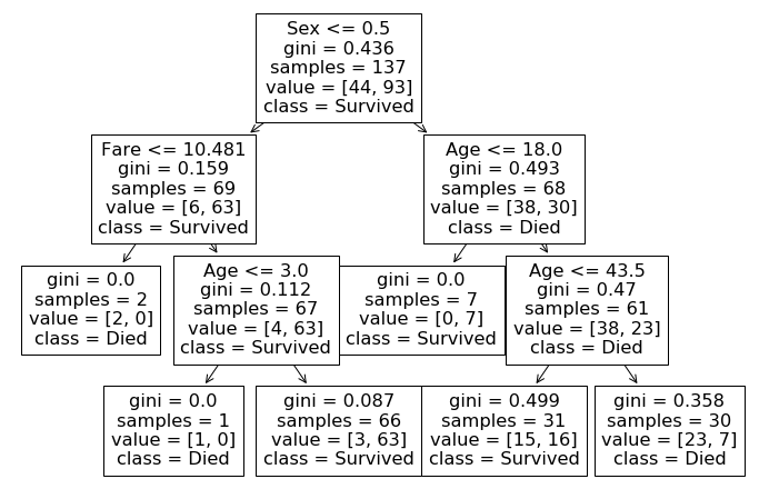
A decision tree makes its decision by trying to find which feature is the most important at each step. Let’s think about how we could do this. Suppose that all the passengers on the Titanic were males (obviously this wasn’t the case, but just bear with me). Then checking whether or not someone was a male would be useless, as it wouldn’t tell us anything. Similarly, if all but just, say, five were males, then that too is not useful. Even if it ended up all females survived, then we’ve only concluded something about five passengers. Therefore, our first task is to choose a feature that has an even balance of samples. If your feature has more than one possible value (like how PClass can be 1, 2, or 3, or how Fare can be any real number), then we also consider a cutoff. So we would want to choose a cutoff for Fare so that there is an even balance of people on each side of the cutoff. For instance, perhaps half the people had a fare more than $20, and half had a fare greater than or equal to $20. Then $20 would be our cutoff.

Let’s start with the entire dataset and see what percentage survived.

df['Survived'].value_counts(normalize=True)

1    0.672131
0    0.327869
Name: Survived, dtype: float64

So about 67.2% of the passengers died, and the remaining 32.8% survived. Suppose you picked a random passenger about which you know nothing whatsoever. You are asked to guess whether or not they died. The best we can do is guess “died” 67.2% of the time, and guess “survived” 32.8% of the time, since that’s all the information we know. If we did so, how often would we be wrong?

Event	Probability	Guessed correct?
Guess survived, actually survived	0.672 * 0.672 = 0.452 (prob. we guess survived * prob. they actually survived)	Yes
Guess survived, actually died	0.672 * 0.328 = 0.220 (prob. we guess survived * prob. they actually died)	No
Guess died, actually survived	0.328 * 0.672 = 0.220	No
Guess died, actually died	0.328 * 0.328 = 0.107	Yes

So we would have guessed incorrectly 0.220 + 0.220 = 0.440 = 44.0% of the time. Not bad, but can we do better if, rather than looking at the entire dataset, we instead split up the data? Let’s split it up by males and females, and consider each separately.

sex_le = label_encoders['Sex']
males_df = df[df['Sex'] == sex_le.transform(['male'])[0]]
females_df = df[df['Sex'] == sex_le.transform(['female'])[0]]

males_df.head()

	PassengerId	Survived	Pclass	Name	Sex	Age	SibSp	Parch	Ticket	Fare	Cabin	Embarked
6	7	0	1	McCarthy, Mr. Timothy J	1	54.0	0	0	17463	51.8625	E46	2
21	22	1	2	Beesley, Mr. Lawrence	1	34.0	0	0	248698	13.0000	D56	2
23	24	1	1	Sloper, Mr. William Thompson	1	28.0	0	0	113788	35.5000	A6	2
27	28	0	1	Fortune, Mr. Charles Alexander	1	19.0	3	2	19950	263.0000	C23 C25 C27	2
54	55	0	1	Ostby, Mr. Engelhart Cornelius	1	65.0	0	1	113509	61.9792	B30	0

females_df.head()

	PassengerId	Survived	Pclass	Name	Age	SibSp	Parch	Ticket	Fare	Cabin	Embarked
1	2	1	1	Cumings, Mrs. John Bradley (Florence Briggs Th...	38.0	1	0	PC 17599	71.2833	C85	0
3	4	1	1	Futrelle, Mrs. Jacques Heath (Lily May Peel)	35.0	1	0	113803	53.1000	C123	2
10	11	1	3	Sandstrom, Miss. Marguerite Rut	4.0	1	1	PP 9549	16.7000	G6	2
11	12	1	1	Bonnell, Miss. Elizabeth	58.0	0	0	113783	26.5500	C103	2
52	53	1	1	Harper, Mrs. Henry Sleeper (Myna Haxtun)	49.0	1	0	PC 17572	76.7292	D33	0

What percentage of each group survived?

males_df['Survived'].value_counts(normalize=True)

0    0.568421
1    0.431579
Name: Survived, dtype: float64

females_df['Survived'].value_counts(normalize=True)

1    0.931818
0    0.068182
Name: Survived, dtype: float64

Let’s do the same calculations as above to find the probability of guessing wrong. But this time, rather than looking at what percentage of the entire set of passengers survived/died, we’ll deal with men and women separately.

Men only

Event	Probability	Guessed correct?
Guess survived, actually survived	0.432 * 0.432 = 0.187	Yes
Guess survived, actually died	0.432 * 0.568 = 0.245	No
Guess died, actually survived	0.568 * 0.432 = 0.245	No
Guess died, actually died	0.568 * 0.568 = 0.323	Yes

Women only

Event	Probability	Guessed correct?
Guess survived, actually survived	0.068 * 0.068 = 0.005	Yes
Guess survived, actually died	0.068 * 0.932 = 0.063	No
Guess died, actually survived	0.932 * 0.068 = 0.063	No
Guess died, actually died	0.932 * 0.932 = 0.869	Yes

So for men only we guessed incorrectly 0.245 + 0.245 = 0.490 = 49.0% of the time, and for women only we guessed incorrectly 0.063 + 0.063 = 0.126 = 12.6% of the time.

Is this better than looking at the whole dataset? It’s a little tricky to tell at first glance, because now we have two percentages, as opposed to just the single percentage of incorrectness we had when we looked at the entire dataset. You may be tempted to average these two percentages and say that we were incorrect (49.0% + 12.6%) / 2 = 30.8% of the time. But that would assume that there are an equal number of men and women. Instead, we’ll take the weighted average of how many of each sex were on board. Let’s check how many of each sex were on board.

df['Sex'].value_counts()

1    95
0    88
Name: Sex, dtype: int64

Looking at the DataFrames above we see that males have a sex value of 1 and females of 0. So there were 95 males and 88 females. Thus there were 95 + 88 = 183 total passengers. Therefore the weighted average for incorrect guesses is given by

\[ \displaystyle\frac{95}{183} \cdot 0.490 + \frac{88}{183} \cdot 0.126 = 0.254 + 0.061 = 0.315 = 31.5\% \]

Thus we expect to guess incorrectly about 31.5% of the time. This is indeed an improvement above looking at the entire dataset, for which we would have guessed incorrectly 44.0% of the time.

So is Sex the “best” column? Following the ideas above, we can define “best” as the column which causes us to guess incorrectly least often. Rather than repeatedly doing this by hand, let’s write a function to do this work for us. Note that if we use a column like Fare which has many different values, we’ll also need to supply a cutoff. So we could (say) split up our passengers by those who paid more or less than \$20.

def pct_guess_incorrectly(df, col, cutoff):
    # Split up the data according to the cutoff
    df_lower = df[df[col] < cutoff]
    df_upper = df[df[col] >= cutoff]
    
    # Find the percentage of survived and died for each subset
    lower_died_pct = df_lower[df_lower['Survived'] == 0].shape[0] / df_lower.shape[0]
    upper_died_pct = df_upper[df_upper['Survived'] == 0].shape[0] / df_upper.shape[0]
    lower_survived_pct = 1 - lower_died_pct
    upper_survived_pct = 1 - upper_died_pct
    
    # Find the percentage of incorrect guesses for each subsets
    # Prob we picked died * prob they survived + prob we picked survived * prob they died
    lower_incorrect_pct = lower_died_pct*lower_survived_pct + lower_survived_pct*lower_died_pct 
    upper_incorrect_pct = upper_died_pct*upper_survived_pct + upper_survived_pct*upper_died_pct
    
    # Find what percentage of the people were in the upper and lower subsets
    pct_lower = df_lower.shape[0] / df.shape[0] 
    pct_upper = df_upper.shape[0] / df.shape[0] 
    
    # Compute the weighted average
    pct_incorrect = pct_lower * lower_incorrect_pct + pct_upper * upper_incorrect_pct
    
    return pct_incorrect

Let’s double-check that our function is giving the same values as we computed by hand for Sex.

# Since male == 1 and female == 0, we'll use a cutoff of 0.5 to split them up
# In fact, any number strictly between 0 and 1 would work just fine
pct_guess_incorrectly(df, 'Sex', 0.5)

0.31580516118911284

Looks good! Let’s now try Pclass. We don’t know what the cutoff should be (the passenger classes are 1, 2, and 3, so we need to put a cutoff to split them up). We could pick a cutoff that puts all of the passenger classes together, such as cutoff=0. We could pick a cutoff which splits class 1 off, such as cutoff=1.5, and so forth. Let’s just compute it for each of them and see what cutoff gives the lowest chance of guessing incorrectly.

# An error is coming...
pclass_cutoffs = [0, 1.5, 2.5, 3.5]

for cutoff in pclass_cutoffs:
    cutoff_pct_incorrect = pct_guess_incorrectly(df, 'Pclass', cutoff)
    print(f'Cutoff = {cutoff}, % incorrect = {100*cutoff_pct_incorrect:.2f}%')

---------------------------------------------------------------------------
ZeroDivisionError                         Traceback (most recent call last)
<ipython-input-162-90fc85e86a0b> in <module>
      3 
      4 for cutoff in pclass_cutoffs:
----> 5     cutoff_pct_incorrect = pct_guess_incorrectly(df, 'Pclass', cutoff)
      6     print(f'Cutoff = {cutoff}, % incorrect = {100*cutoff_pct_incorrect:.2f}%')

<ipython-input-158-21b216d99eb0> in pct_guess_incorrectly(df, col, cutoff)
      5 
      6     # Find the percentage of survived and died for each subset
----> 7     lower_died_pct = df_lower[df_lower['Survived'] == 0].shape[0] / df_lower.shape[0]
      8     upper_died_pct = df_upper[df_upper['Survived'] == 0].shape[0] / df_upper.shape[0]
      9     lower_survived_pct = 1 - lower_died_pct

ZeroDivisionError: division by zero

Uh-oh, it looks like we’re dividing by zero somewhere! Why would this be? What’s happening is that (at least) one of our cutoffs is producing an empty subset of passengers. For example, there are no passengesr with a Pclass < 0. We didn’t take this into account when we wrote our function, so let’s fix it now by telling the user if they picked a bad cutoff.

def pct_guess_incorrectly(df, col, cutoff):
    # Split up the data according to the cutoff
    df_lower = df[df[col] < cutoff]
    df_upper = df[df[col] >= cutoff]
    
    # If either of these subsets is empty, set the percentages to zero
    if df_lower.shape[0] == 0 or df_upper.shape[0] == 0:
        print(f'Cutoff of {cutoff} for column {col} produced an empty subset, change the cutoff')
        return None
    
    # Find the percentage of survived and died for each subset
    lower_died_pct = df_lower[df_lower['Survived'] == 0].shape[0] / df_lower.shape[0]
    upper_died_pct = df_upper[df_upper['Survived'] == 0].shape[0] / df_upper.shape[0]
    lower_survived_pct = 1 - lower_died_pct
    upper_survived_pct = 1 - upper_died_pct
    
    # Find the percentage of incorrect guesses for each subsets
    # Prob we picked died * prob they survived + prob we picked survived * prob they died
    lower_incorrect_pct = lower_died_pct*lower_survived_pct + lower_survived_pct*lower_died_pct 
    upper_incorrect_pct = upper_died_pct*upper_survived_pct + upper_survived_pct*upper_died_pct
    
    # Find what percentage of the people were in the upper and lower subsets
    pct_lower = df_lower.shape[0] / df.shape[0] 
    pct_upper = df_upper.shape[0] / df.shape[0] 
    
    # Compute the weighted average
    pct_incorrect = pct_lower * lower_incorrect_pct + pct_upper * upper_incorrect_pct
    
    return pct_incorrect

pclass_cutoffs = [0, 1.5, 2.5, 3.5]

for cutoff in pclass_cutoffs:
    cutoff_pct_incorrect = pct_guess_incorrectly(df, 'Pclass', cutoff)
    if cutoff_pct_incorrect is not None:
        print(f'Cutoff = {cutoff}, % incorrect = {100*cutoff_pct_incorrect:.2f}%')

Cutoff of 0 for column Pclass produced an empty subset, change the cutoff
Cutoff = 1.5, % incorrect = 44.07%
Cutoff = 2.5, % incorrect = 43.73%
Cutoff of 3.5 for column Pclass produced an empty subset, change the cutoff

So it looks like grouping by passenger class is not an improvement over grouping by sex. Let’s try Fare next. Since there are so many possible fares, we’ll just create a really big list of cutoffs and let the code find which one is best. The simplest way to create a big list of evenly spaced points is to use linspace() from numpy. This creates linearly spaced points (hence the name). It wants to know the starting and ending points, and how many points you want in-between. Here’s an example:

# Starts at 0, ends at 5, creates 10 evenly spaced points in-between
np.linspace(0, 5, 10)

array([0.        , 0.55555556, 1.11111111, 1.66666667, 2.22222222,
       2.77777778, 3.33333333, 3.88888889, 4.44444444, 5.        ])

# Create cutoffs for the entire range of fares, and generate 1000 different cutoffs
fare_cutoffs = np.linspace(df['Fare'].min(), df['Fare'].max(), 1000)

# Keep track of what cutoff produced the lowest percentage of incorrect guesses
best_pct_incorrect = 1
best_cutoff = None

# Go through all cutoffs
for cutoff in fare_cutoffs:
    cutoff_pct_incorrect = pct_guess_incorrectly(df, 'Fare', cutoff)
    # Check if it worked (didn't return a None), and if the % incorrect is lower than what we've seen so far
    if cutoff_pct_incorrect is not None and cutoff_pct_incorrect < best_pct_incorrect:
        # If so, save it
        best_pct_incorrect = cutoff_pct_incorrect
        best_cutoff = cutoff
        
# Print out the results
print(f'Best cutoff = {best_cutoff:.3f} had a % incorrect of {100*best_pct_incorrect:.2f}%')

Cutoff of 0.0 for column Fare produced an empty subset, change the cutoff
Best cutoff = 7.693 had a % incorrect of 41.01%

So a cutoff of $7.69 produced the best outcome with 41.01% of the guesses being incorrect. This is still worse than we got with the Sex column.

Certainly we could repeat this for all columns, but hopefully at this point you get the idea. In fact, Sex will produce the best results, as we know by looking at the decision tree we built! The decision trees go through this process for all columns and for all possible cutoffs. It then picks which one got the best result (lower percentage chance of guessing incorrectly) and chooses that as the first node. It then repeats this process for each node in the tree until the specificied max_depth is reached.

The value we have been calling “percentage guessed incorrectly” is really called the Gini impurity. If you look at the sklearn decision tree documentation you will see a parameter called “criterion”, which has a default value of “gini”. This means that the criteria it uses to form the tree is Gini impurity. You now understand how decision trees work!

Exercises¶

Grab another dataset and make your own decision trees. How do changing the hyperparameters affect the result?
Write a function which goes through all possible columns and all cutoffs and finds which gives the best (lowest) Gini impurity.
In the sklearn decision tree documentation there are many other hyperparameters you can choose. Read about them and try playing with them.

Introduction to Data Science